[ELDA] [Paper] Optimizing Data Pipelines for Machine Learning in Feature Stores

Paper published in VLDB 2022

Overview

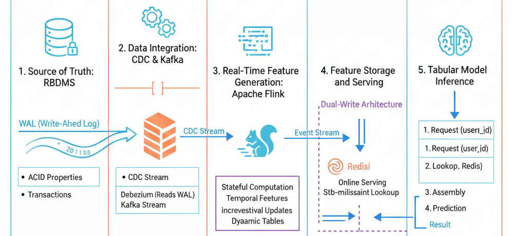
Paper introduces FeathrPO (Feathr Pipeline Optimization), a system designed to optimize Feature Stores (FS). While current Feature Stores function well as a “DBMS-for-ML,” they are often resource-hungry and lack database-style optimizations.

The paper identifies that the Point-in-Time (PIT) Join (also known as ASOF join) is the most critical and expensive operation in feature pipelines. To address this, FeathrPO proposes optimizations in two key areas: Feature Computation Reuse and Data Source Layout.

Background: Point-in-Time (PIT) Join

What is a Point-in-Time Join?

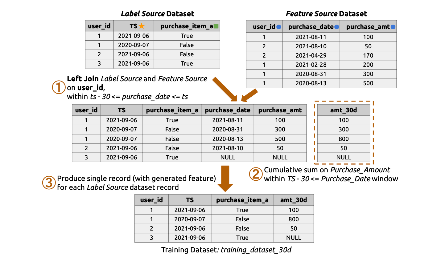
The Point-in-Time Join (often referred to as a PIT join or ASOF join) is the cornerstone operation in Feature Stores for generating correct training datasets. Unlike a standard database join that matches records based solely on key equality (e.g., User ID), a PIT join introduces a temporal constraint to ensure that features accurately reflect the state of the world at a specific historical moment.

Why is it Critical? (The Data Leakage Problem)

The primary purpose of a PIT join is to prevent data leakage—one of the most destructive issues in machine learning pipelines.

Data leakage occurs when information from the future (relative to the prediction time) accidentally “leaks” into the training set. For example, if you are training a model to predict whether a user will churn in October, you strictly cannot use customer support logs from November. If you do, the model will “cheat” during training but fail in production where future data is unavailable.

The PIT join strictly enforces this by ensuring that for every training label (an event we want to predict), we only join features that were available at or before that specific timestamp.

How It Works: A Conceptual Example

Consider an e-commerce scenario where we want to predict if a customer will buy a specific item during Labor Week 2022.

Label Dataset (The Target): This contains the “ground truth” we are trying to predict.
- Record: User A, Timestamp: 2022-09-06 (Labor Day), Target: True (Bought Item).
Feature Dataset (The History): This contains raw historical logs, such as daily purchase amounts.
- Record 1: User A, 2022-08-11, Amount: $50
- Record 2: User A, 2022-09-08, Amount: $100 (Future Data!)

A standard join might erroneously include the $100 purchase from September 8th because it matches “User A”. A Point-in-Time Join, however, looks at the label timestamp (2022-09-06) and filters the feature history to only include records where purchase_date <= 2022-09-06.

1. Reuse-Based Feature Computation

Machine Learning development is iterative. Data scientists frequently generate training datasets with slightly different parameters (e.g., changing a time window from 30 days to 40 days) to tune models. FeathrPO automates the reuse of previously materialized features to accelerate these new computations.

A. Incremental Query Rewriting

Instead of computing a new feature request from scratch, FeathrPO rewrites the feature generation SQL to treat the new request as an “incremental update” to an existing view.

Case Example:

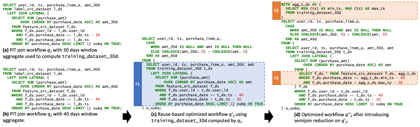
Existing Feature ($q_1$): A user has already computed a training dataset with a 30-day window aggregate (amt_30d).
New Request ($q_2$): The user wants to test if a 40-day window (amt_40d) improves model accuracy.
Optimization: FeathrPO rewrites the query for $q_2$ to use the materialized results of $q_1$ (training_dataset_30d) as the base table. The inner subquery is modified to scan only the “delta” (the extra 10 days of data) from the raw source, rather than scanning the full 40 days again.

B. Semi-Join Reduction

To further optimize the “delta” computation, FeathrPO applies a semi-join reduction technique.

Mechanism: The system computes the minimum and maximum timestamps from the existing training dataset ($q_1$).
Result: These timestamp bounds are pushed down as filters to the raw feature source scan. This “semi-join” logic aggressively prunes data that falls outside the relevant time range, significantly reducing I/O.

2. Automatic Layout Selection

Feature pipelines heavily rely on time-series data, where queries typically filter by a time dimension. Standard storage layouts often force the compute engine to scan excessive amounts of irrelevant data. FeathrPO moves beyond simple static partitioning by introducing an automatic, workload-aware layout selector.

A. Candidate Generation (The Flooring Function)

Instead of guessing the best partition key, the system automatically proposes strategies based on the specific access patterns of the feature workload. It uses a flooring function $f(t, e)$ to generate candidate layouts for a timestamp column $t$.

Granularity Levels ($e$): The system evaluates four specific levels of temporal granularity:
- Year
- Month
- Day
- Hour
Example: If a dataset is frequently accessed with 3-day lookback windows, the system identifies that partitioning by Day or Hour might offer better pruning than Month.

B. Global Selection via Binary Integer Programming (BIP)

Unlike standard database optimizers that optimize one query at a time, FeathrPO performs global optimization. It analyzes the history of all pipelines to find a single layout that works best for the entire workload.

The Optimization Problem: The system formulates the layout selection as a mathematical problem to be solved by a Binary Integer Programming (BIP) solver.
- Objective: Minimize the global sum of data scanned across all pipelines.
- Constraint 1 (Uniqueness): Each dataset can only have one physical layout (e.g., you cannot partition by both Day and Month simultaneously).
- Constraint 2 (Reconfiguration Budget $B$): Crucially, the system respects a “budget” that limits the total volume of data that can be rewritten during a reorganization cycle. This prevents the system from proposing expensive changes (like rewriting Petabytes of data) for only marginal performance gains.

C. Cost Estimation with KLL Sketches

To solve this BIP problem efficiently without reading the actual data, FeathrPO uses KLL Sketches (a type of quantile sketch).

Partition Elimination: The sketches allow the optimizer to estimate the data distribution and accurately predict how many partitions can be skipped (partition elimination) for any given candidate strategy.
Efficiency: This enables the system to evaluate thousands of candidate layouts and queries in seconds.