The following notes summarize my understanding of TabICL based on reading its source code , with additional clarification inspired by Claude’s explanations.

1. Architecture Overview

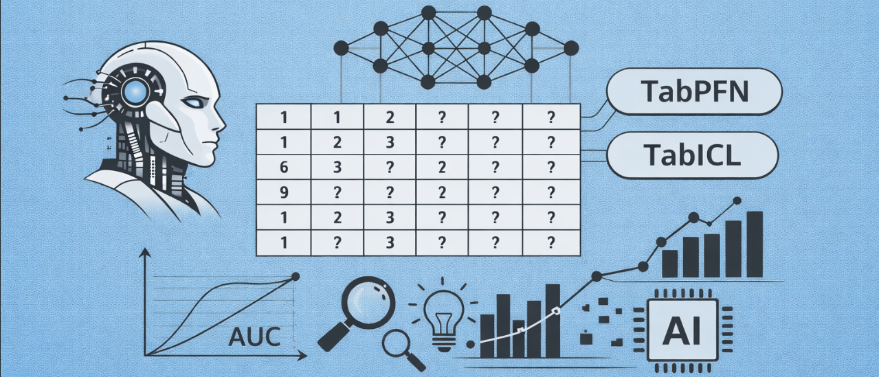
Model: TabICL (Tabular In-Context Learning)

Default Configuration:

• Embedding dimension: 128
• Column embedding: 3 blocks, 4 heads, 128 inducing points
• Row interaction: 3 blocks, 8 heads, 4 CLS tokens
• ICL predictor: 12 blocks, 4 heads
• Max classes: 10 (with automatic hierarchical classification for more)
• Feedforward factor: 2
• Positional embedding: RoPE (Rotary Position Encoding) for row interaction

Complete Pipeline

Input: X_train (100, 10) + X_test (50, 10), y_train (100,)
    ↓
Stage 1: Column-wise Embedding (Distribution-Aware)
    Linear Projection (shared across columns)
        Shape: (B, 150, 10) → (B, 10, 150, 1) → (B, 10, 150, 128)
    Set Transformer (3 blocks with 128 inducing points)
        Generates distribution-aware weights and biases
    Feature-specific Transformation
        embeddings = features * weights + biases
        Shape: (B, 10, 150, 128) → (B, 150, 14, 128)
        Note: 14 = 10 features + 4 CLS tokens
    ↓
Stage 2: Row-wise Interaction (Context-Aware)
    Prepend CLS tokens (4 learnable tokens per row)
    Encoder with RoPE (3 blocks, 8 heads)
        Shape: (B, 150, 14, 128)
    Extract & Concatenate CLS tokens
        Shape: (B, 150, 4×128) → (B, 150, 512)
    ↓
Stage 3: Dataset-wise In-Context Learning
    Add label embeddings to training samples
        y_train → OneHot → Linear(10, 512)
        R[:, :100] = R[:, :100] + y_encoder(y_train)
    ICL Transformer (12 blocks, 4 heads)
        Training samples attend to themselves
        Test samples attend only to training samples
        Shape: (B, 150, 512)
    Decoder MLP (2-layer with GELU)
        Shape: (B, 50, 512) → (B, 50, 1024) → (B, 50, 10)
    ↓
Softmax → Argmax → Label Decoding
    Output: (50,) — predicted classes

Three-Stage Design Philosophy

Each stage serves a distinct purpose:

1. Column-wise Embedding: Captures distributional properties within each feature
   • Uses Set Transformer with inducing points for O(n) complexity
   • Learns feature-specific transformations based on column statistics
   • Shared weights across features enable generalization
2. Row-wise Interaction: Captures feature interactions within each sample
   • Uses rotary position encoding to preserve feature order
   • CLS tokens aggregate information from all features
   • Enables the model to learn complex feature relationships
3. Dataset-wise ICL: Learns task-specific patterns from labeled examples
   • Training samples receive label information
   • Test samples attend to training samples for in-context learning
   • Supports hierarchical classification for datasets with >10 classes

2. Stage 1: Column-wise Embedding

Purpose: Distribution-Aware Feature Representation

Unlike traditional approaches that use separate embedding layers per column, TabICL employs a shared Set Transformer to process all features. This enables the model to learn distributional properties and generate feature-specific transformations.

Step 1: Linear Projection

Each scalar cell is first projected into the embedding space:

# Shared linear layer for all features
in_linear = SkippableLinear(1, 128)

# Reshape: (B, T, H) → (B, H, T, 1)
features = X.transpose(1, 2).unsqueeze(-1)

# Project: (B, H, T, 1) → (B, H, T, 128)
src = in_linear(features)

Shape: (B, 10, 150, 1) → (B, 10, 150, 128)

Step 2: Set Transformer with Induced Self-Attention

The Set Transformer processes each feature column independently using induced self-attention:

# 3 blocks of induced self-attention
# Each block has 128 learnable inducing points
SetTransformer(
    num_blocks=3,
    d_model=128,
    nhead=4,
    num_inds=128,
    dim_feedforward=256
)

Induced Self-Attention reduces complexity from O(n²) to O(n):

Standard self-attention requires each of n samples to attend to all n samples (n² operations). Induced self-attention uses m learnable inducing points (m=128) as an information bottleneck to reduce this to O(m·n) operations.

Two-Stage Attention Process:

Stage 1: Aggregate                    Stage 2: Distribute
Inducing Points ← Samples             Samples ← Inducing Points

  128 inducing points                   150 samples
       ↑ ↑ ↑                               ↑ ↑ ↑
       | | |                               | | |
  150 samples                          128 inducing points

Complexity: O(128 × 150)              Complexity: O(150 × 128)

Stage 1 - Aggregate: Each of the 128 inducing points attends to all n samples

hidden = attention(
    query=inducing_points,    # (128, 128)
    key=samples,              # (150, 128)
    value=samples             # (150, 128)
)
# Inducing points collect global information from the entire column

Stage 2 - Distribute: Each sample attends to the 128 inducing points

output = attention(
    query=samples,            # (150, 128)
    key=hidden,               # (128, 128)
    value=hidden              # (128, 128)
)
# Each sample retrieves relevant global patterns from inducing points

Complexity Comparison (for a column with 10,000 samples):

• Standard attention: 10,000² = 100,000,000 operations
• Induced attention: 2 × 128 × 10,000 = 2,560,000 operations (~40× faster)

Information Leakage Prevention: During inference, if train_size is specified, Stage 1 is restricted so inducing points only attend to training samples. Stage 2 remains unrestricted, allowing test samples to query the inducing points. This ensures inducing points learn patterns only from training data while still allowing test samples to benefit from these learned patterns.

Step 3: Distribution-Aware Transformation

The Set Transformer outputs are used to generate weights and biases for each feature:

# Generate weights and biases from transformer output
weights = out_w(src)  # (B, H, T, 128)
biases = out_b(src)   # (B, H, T, 128)

# Apply feature-specific transformation
embeddings = features * weights + biases

This allows the model to:

• Adapt to the distribution of values within each column
• Handle different scales and ranges automatically
• Learn column-specific patterns

Step 4: Reserve Space for CLS Tokens

# Pad with -100.0 to reserve slots for CLS tokens
X = nn.functional.pad(X, (4, 0), value=-100.0)

The -100.0 value marks positions that should be skipped in SkippableLinear and SetTransformer, and will later be filled with learnable CLS tokens in the row interaction stage.

Complete Example

Input:
  X = [1.5, 2.3, 0.8, ..., 4.1]  # 10 features for 150 samples

After Linear Projection (shared):
  All cells → 128-dim vectors

After Set Transformer (per column):
  Column 0: Processes all 150 values → learns distribution
  Column 1: Processes all 150 values → learns distribution
  ...
  Generates weights & biases for each column

After Transformation:
  Column 0: [1.5] * w0 + b0 = [0.15, -0.23, ..., 0.42]
  Column 1: [2.3] * w1 + b1 = [0.31, 0.08, ..., -0.17]
  ...

Output:
  Shape: (B, 150, 14, 128)  # 10 features + 4 reserved CLS slots

3. Stage 2: Row-wise Interaction

Purpose: Context-Aware Feature Interaction

This stage captures interactions between features within each row using a transformer encoder with Rotary Position Encoding (RoPE). It uses learnable CLS tokens to aggregate information from all features.

Step 1: Prepend CLS Tokens

# 4 learnable CLS tokens (initialized per row)
cls_tokens = nn.Parameter(torch.empty(4, 128))

# Insert at the beginning of each row
embeddings[:, :, :4] = cls_tokens.expand(B, T, 4, 128)

Shape: (B, 150, 14, 128) where positions 0-3 are CLS tokens

Step 2: Encoder with Rotary Position Encoding

# Encoder: 3 blocks of multi-head attention with RoPE
Encoder(
    num_blocks=3,
    d_model=128,
    nhead=8,
    dim_feedforward=256,
    use_rope=True,
    rope_base=100000
)

Why RoPE:

• Makes feature positions distinguishable to enable ensemble diversity through feature shuffling
• Without position encoding, all feature orderings would produce identical outputs
• No learned positional parameters (purely geometric encoding)
• Generalizes to variable number of features

Attention Pattern:

• Each feature attends to all other features in the same row
• CLS tokens collect global information from all features
• RoPE ensures different feature orderings create different predictions

Step 3: Extract and Concatenate CLS Tokens

# Extract only CLS token outputs
cls_outputs = outputs[:, :, :4, :]  # (B, 150, 4, 128)

# Apply layer norm (if pre-norm architecture)
cls_outputs = ln(cls_outputs)

# Concatenate CLS tokens into a single vector per row
representations = cls_outputs.flatten(-2)  # (B, 150, 512)

The concatenated CLS tokens form the final row representation with dimension 4 × 128 = 512.

Complete Example

Input (after Stage 1):
  Row 0: [CLS0, CLS1, CLS2, CLS3, Feat0, Feat1, ..., Feat9]
         Each is a 128-dim vector

After Encoder with RoPE:
  - Feat0 attends to all other features with position awareness
  - CLS tokens aggregate information from all features
  - Output: (B, 150, 14, 128)

After Extraction:
  - Keep only CLS tokens: (B, 150, 4, 128)
  - Concatenate: (B, 150, 512)

Result:
  Each row is now represented by a 512-dim vector
  This vector encodes feature interactions and global row information

4. Stage 3: Dataset-wise In-Context Learning

Purpose: Learn from Labeled Examples

This stage implements in-context learning by conditioning the model on training examples to make predictions on test samples.

Step 1: Label Encoding for Training Samples

# One-hot encode labels and project to embedding space
y_encoder = OneHotAndLinear(max_classes=10, embed_dim=512)

# Add label information to training samples only
R[:, :train_size] = R[:, :train_size] + y_encoder(y_train)

• Training samples receive their label embeddings
• Test samples remain unchanged
• This conditions the model on the task

Step 2: ICL Transformer with Split Attention

# Encoder: 12 blocks of multi-head attention
Encoder(
    num_blocks=12,
    d_model=512,
    nhead=4,
    dim_feedforward=1024
)

# Special attention mask: attn_mask=train_size
# - Training samples attend to each other
# - Test samples attend ONLY to training samples

Split Attention Pattern:

       Train-0  Train-1  ...  Train-99  Test-0  Test-1  ...  Test-49
Train-0   ✓       ✓      ...     ✓        ✗       ✗     ...    ✗
Train-1   ✓       ✓      ...     ✓        ✗       ✗     ...    ✗
...
Train-99  ✓       ✓      ...     ✓        ✗       ✗     ...    ✗
Test-0    ✓       ✓      ...     ✓        ✗       ✗     ...    ✗
Test-1    ✓       ✓      ...     ✓        ✗       ✗     ...    ✗
...
Test-49   ✓       ✓      ...     ✓        ✗       ✗     ...    ✗

This ensures:

• Training samples establish context through self-attention
• Test samples learn patterns by attending to labeled training samples
• No information leakage between test samples

Step 3: Decoder MLP

decoder = nn.Sequential(
    nn.Linear(512, 1024),  # Expand
    nn.GELU(),
    nn.Linear(1024, 10)    # Project to class logits
)

# Extract test sample encodings
test_encodings = output[:, train_size:, :]  # (B, 50, 512)

# Decode to class logits
logits = decoder(test_encodings)  # (B, 50, 10)

Step 4: Prediction

# Apply softmax with temperature
probs = softmax(logits / temperature)  # (B, 50, 10)

# Select most likely class
predictions = argmax(probs, dim=-1)  # (B, 50)

Hierarchical Classification (>10 Classes)

When the number of classes exceeds 10, TabICL automatically uses hierarchical classification:

# Example: 25 classes
# Level 0 (Root): 25 classes → 3 groups [9, 8, 8]
#   Level 1 (Group 0): 9 classes → predict directly
#   Level 1 (Group 1): 8 classes → predict directly
#   Level 1 (Group 2): 8 classes → predict directly

# Prediction combines probabilities via chain rule:
# P(class_i) = P(group_j) × P(class_i | group_j)

How it works:

1. Build tree: Partition classes into balanced groups (≤10 per level)
2. Predict groups: Use ICL to classify into groups at each level
3. Combine probabilities: Multiply probabilities down the tree
4. Return final: Probabilities over all original classes

Complete Example

Input: R_train (100, 512), R_test (50, 512), y_train (100,)

Step 1: Add Label Embeddings
  R_train[0] = R_train[0] + y_encoder(y_train[0])  # e.g., class 2
  R_train[1] = R_train[1] + y_encoder(y_train[1])  # e.g., class 0
  ...
  R_test[0] = R_test[0]  # No label information

Step 2: ICL Transformer
  Concatenate: [R_train; R_test] → (150, 512)
  Process with split attention (train_size=100)
  Output: (150, 512)

Step 3: Decode Test Samples
  test_out = output[100:, :]  # (50, 512)
  logits = decoder(test_out)  # (50, 10)

  Example logits: [-1.2, 0.5, 3.2, -0.8, 0.1, ...]

Step 4: Softmax & Argmax
  probs = softmax([-1.2, 0.5, 3.2, ...] / 0.9)
       = [0.02, 0.09, 0.78, 0.03, 0.05, ...]

  prediction = argmax([0.02, 0.09, 0.78, ...]) = 2

Result:
  Predicted class = 2
  Matches training sample 0's label!

5. Key Design Choices

Why Three Stages?

1. Column-wise: Learn what each feature means independently
2. Row-wise: Learn how features interact within samples
3. Dataset-wise: Learn the specific prediction task

This modular design allows each stage to specialize while maintaining end-to-end differentiability.

Why Set Transformer for Column Embedding?

• Permutation invariance: Order of samples doesn’t matter
• Efficiency: O(n) complexity via inducing points
• Distribution awareness: Learns from all values in a column
• Shared weights: Generalizes across different feature types

Why RoPE for Row Interaction?

• Feature slot identification: Makes positions distinguishable so feature shuffling creates diverse ensemble members
• Ensemble diversity: Without positional encoding, different feature orderings would yield identical predictions
• Generalization: Works with variable number of features
• No learned parameters: Purely geometric encoding

Why CLS Tokens?

• Aggregation: Collect information from all features
• Fixed size: Produces consistent output regardless of feature count
• Flexibility: Multiple tokens capture different aspects
• Efficiency: Avoid processing all feature embeddings downstream

Why Split Attention for ICL?

• In-context learning: Test samples learn from training examples
• No leakage: Test samples can’t cheat by seeing each other
• Task adaptation: Different training sets → different predictions
• Efficiency: Single forward pass handles train + test together

6. Comparison with TabPFN

Aspect	TabPFN	TabICL
Architecture	Dual attention (feature-wise + item-wise)	Three-stage (column + row + ICL)
Positional Encoding	Subspace embedding (learned)	RoPE (geometric)
Column Embedding	Shared linear layer + fixed positional encoding	Set Transformer with distribution-aware transformation
Max Samples	~1,000	60,000+ (with memory management)
Max Features	~100	100+
Max Classes	10	10+ (with hierarchical classification)
Complexity	O(n²) per stage	O(n) for column, O(n²) for row & ICL
Focus	Small data, fast inference	Large data, scalability