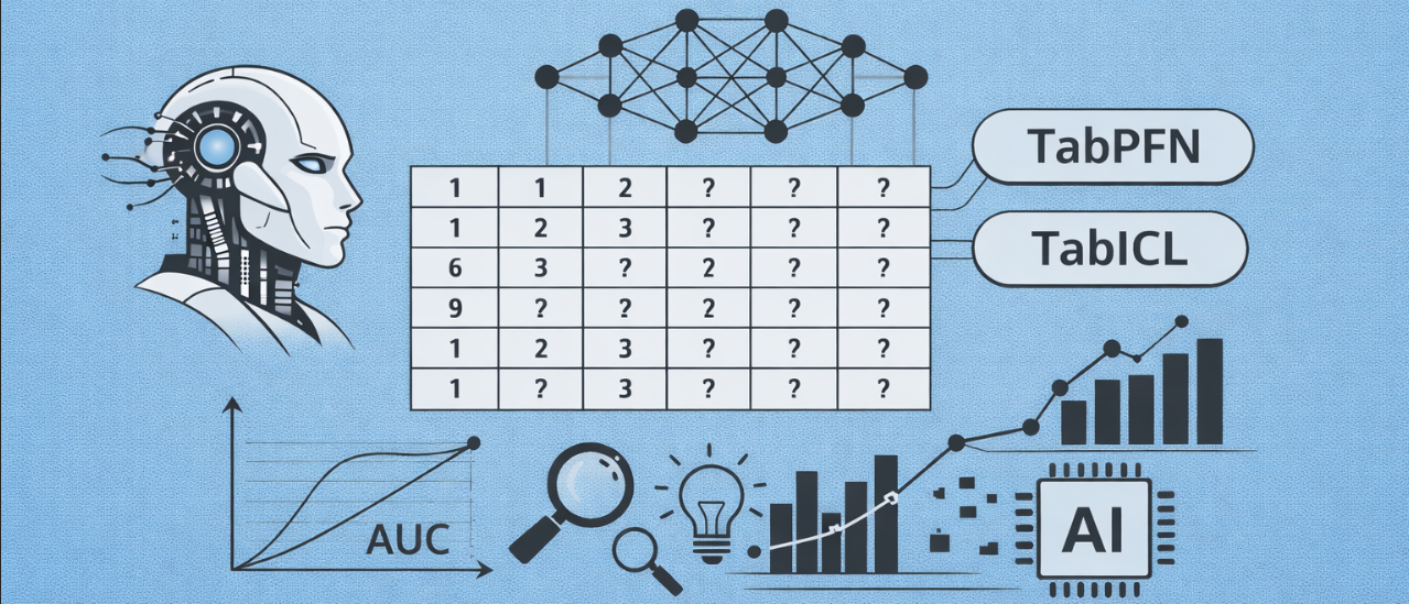
The following notes summarize my understanding of TabICL based on reading its source code , with additional clarification inspired by Claude’s explanations. In TabPFN, the code of data generation is not released, but the details is described in paper Appendix.C. However, the following implementation in tabICL should be more make sense in my perspective.

1. Overview

TabICL is trained on synthetic tabular datasets generated using Structural Causal Models (SCM). The key insight: use randomly initialized neural networks to create realistic causal structures without requiring real data.

The code of data generation is save in repository src/prior.

Why Synthetic Data?

• Infinite diversity: Generate unlimited datasets with different structures
• Controllable properties: Specify features, samples, classes, complexity
• No privacy concerns: No real-world data needed
• Universal patterns: Learn to handle any data structure

Two Generation Methods

1. MLP-based SCM (mlp_scm.py): Uses Multi-Layer Perceptrons with random weights
2. Tree-based SCM (tree_scm.py): Uses tree models (RandomForest, XGBoost) fitted to random noise

Both create complex, non-linear feature relationships that mimic real-world data.

1.Structural Causal Models

Real-World Intuition

In real datasets, features are not independent - they share common underlying causes:

Medical Data Example:

Root Causes (unobserved):
  - Genetics
  - Lifestyle
  - Environment
    ↓
Intermediate Effects:
  - Inflammation levels
  - Hormone levels
  - Blood chemistry
    ↓
Observable Features:
  - Blood pressure
  - Cholesterol
  - Heart rate
  - BMI
    ↓
Target:
  - Disease diagnosis

Key insight: Features we measure are snapshots from different stages of an underlying causal process.

SCM Simulation

Instead of having real causes, we simulate the causal process:

Random Root Variables
    ↓
Layer 1 transformations
    ↓
Layer 2 transformations
    ↓
...
    ↓
Layer N transformations
    ↓
Sample features from different layers

This creates realistic correlations because features share common causal ancestors.

3. MLP-Based Data Generation (Step-by-Step)

Step 1: Sample Root Causes

# Generate initial cause variables
xsampler = XSampler(
    seq_len=1024,        # Number of samples (rows)
    num_causes=10,       # Number of root variables
    sampling="mixed"     # Normal, uniform, categorical, or Zipf distributions
)

causes = xsampler.sample()  # Shape: (1024, 10)

What this creates:

• 1024 samples (dataset rows)
• Each sample has 10 root cause variables
• Can be normal distribution, uniform, categorical, or power-law

Step 2: Build Causal Chain with Random MLP

IMPORTANT: The MLP weights are randomly initialized and never trained.

mlp = MLPSCM(
    seq_len=1024,
    num_features=100,      # Final number of features
    num_outputs=1,         # Number of target variables
    num_layers=10,         # Depth of causal chain
    hidden_dim=200,        # Intermediate variables per layer
    init_std=1.0,          # Random initialization std
    noise_std=0.01         # Gaussian noise std
)

Architecture:

Layer 0: Linear(10 → 200)                    [Random weights]
Layer 1: Tanh → Linear(200 → 200) → Noise   [Random weights]
Layer 2: Tanh → Linear(200 → 200) → Noise   [Random weights]
...
Layer 9: Tanh → Linear(200 → 200) → Noise   [Random weights]

Forward pass through random MLP:

x = causes  # (1024, 10)
outputs = []

# Layer 0: Initial projection
x = Linear_0(x)  # (1024, 10) → (1024, 200)
outputs.append(x)

# Layers 1-9: Repeated transformations
for i in range(1, 10):
    x = Tanh(x)
    x = Linear_i(x)              # (1024, 200) → (1024, 200)
    x = x + N(0, 0.01)           # Add Gaussian noise
    outputs.append(x)            # Save intermediate output

# Skip first two outputs (causes and first linear)
outputs = outputs[2:]  # Keep 9 layers

Result: 9 tensors, each of shape (1024, 200)

---

Understanding the Dimensions

After Layer 2-10, we have:

outputs[0] = (1024, 200)  ← Layer 2 output (early effects)
outputs[1] = (1024, 200)  ← Layer 3 output
outputs[2] = (1024, 200)  ← Layer 4 output
...
outputs[8] = (1024, 200)  ← Layer 10 output (late effects)

What each dimension means:

• 1024: Number of samples (rows in dataset)
• 200: Number of intermediate variables at this layer
• 9 tensors: Different stages of the causal process

The 9 represents causal depth (how many transformation stages), NOT the number of features.

---

Step 3: Sample Features from Causal Graph

Flatten all intermediate outputs into a single pool:

# Concatenate all 9 layers
outputs_flat = torch.cat(outputs, dim=-1)
# Shape: (1024, 9 × 200) = (1024, 1800)

This creates a pool of 1800 intermediate variables:

Sample 0: [h_0, h_1, h_2, ..., h_199, h_200, ..., h_1799]
           └─ Layer 2 (0-199) ─┘ └─ Layer 3 (200-399) ─┘  ... └─ Layer 10 ─┘

Each h_i represents a variable at a specific stage in the causal chain:

• h_0 to h_199: Early effects (Layer 2)
• h_200 to h_399: Layer 3 effects
• …
• h_1600 to h_1799: Late effects (Layer 10)

Randomly select features:

# Random permutation of indices 0-1799
random_perm = torch.randperm(1800)
# Example: [523, 12, 1205, 899, 34, ..., 1799]

# Select 100 features (skip first for target)
indices_X = random_perm[1:101]
X = outputs_flat[:, indices_X]  # (1024, 100)

# Select target (usually from late effects)
if y_is_effect:
    y = outputs_flat[:, -1]      # Last variable (late effect)
else:
    y = outputs_flat[:, random_perm[0]]  # Random variable

What this means:

# For all 1024 samples:
X[:, 0] = h_12      ← Feature 0 from Layer 2 (early)
X[:, 1] = h_1205    ← Feature 1 from Layer 7 (late)
X[:, 2] = h_899     ← Feature 2 from Layer 5 (mid)
...
X[:, 99] = h_777    ← Feature 99 from Layer 4

y = h_1799          ← Target from Layer 10 (late effect)

Can all features come from Layer 2?

• Technically yes, but extremely unlikely (~10^-150 probability)
• Typically get ~11 features per layer on average
• This diversity creates datasets with varying complexity

---

Step 4: Convert to Classification

# Step 4a: Convert some features to categorical
for i in range(100):
    if random.random() < 0.3:  # 30% of features
        num_bins = random.randint(2, 20)
        X[:, i] = digitize(X[:, i], bins=num_bins)

# Step 4b: Standardize continuous target
y = (y - mean(y)) / std(y)

# Step 4c: Convert to classes using rank-based method
y_sorted = argsort(y)
samples_per_class = 1024 // 10  # ~102 per class

for class_idx in range(10):
    start = class_idx * samples_per_class
    end = (class_idx + 1) * samples_per_class
    y[y_sorted[start:end]] = class_idx

Result:

Original y (continuous): [-2.3, 0.5, 1.8, -0.3, ...]
                           ↓
After classification:     [0, 5, 9, 2, ...]  (10 classes)

---

Step 5: Train/Test Split

# Randomly sample split position (10%-90% of data)
train_size = random.randint(102, 921)  # e.g., 600

# Dataset structure:
# X[:train_size]    = Training features
# y[:train_size]    = Training labels
# X[train_size:]    = Test features
# y[train_size:]    = Test labels (to predict)

---

4. Why Random Weights? (No Training!)

The Surprising Truth

The MLP is NEVER trained with gradients. Weights remain random throughout.

# Step 1: Create MLP with random weights
mlp = MLPSCM(...)  # Random initialization

# Step 2: Use immediately to generate data
X, y = mlp()  # Forward pass only!

# Step 3: Discard this MLP
del mlp

# Step 4: Create NEW MLP with different random weights for next dataset
mlp2 = MLPSCM(...)  # Different random weights
X2, y2 = mlp2()

No optimizer. No loss. No backward(). No training.

Why This Works

Based on established deep learning theory:

1. Random Features Theory (Rahimi & Recht, 2007): Random projections can approximate complex kernel functions, preserving meaningful structure even without training.

2. Neural Tangent Kernels (NTK) (Jacot et al., 2018): In the infinite-width limit, randomly initialized neural networks behave like kernel methods and compute well-defined functions.

3. Lottery Ticket Hypothesis (Frankle & Carbin, 2019): Random networks contain useful subnetworks that can perform complex computations.

4. Biological Plausibility: Random connectivity is observed in biological neural networks and provides computational advantages.

Example

# Two random MLPs with same architecture, different weights
torch.manual_seed(42)
mlp1 = MLPSCM(num_features=100, num_layers=9)
X1, y1 = mlp1()  # Dataset 1

torch.manual_seed(999)
mlp2 = MLPSCM(num_features=100, num_layers=9)
X2, y2 = mlp2()  # Dataset 2

# X1 and X2 have:
# - Same dimensions (100 features, 1024 samples)
# - Different feature relationships (different random weights)
# - Different causal structures
# - Different classification boundaries

This diversity is exactly what TabICL needs to learn universal patterns!

5. Why Add Gaussian Noise?

The Problem Without Noise

# Deterministic MLP (no noise)
causes = [0.5, -1.2, 0.8, ...]
  ↓ MLP
X = [2.3, -0.5, 1.1, ...]  # Always the same output
y = 1.234

# If another sample has identical causes:
causes = [0.5, -1.2, 0.8, ...]  # Same!
  ↓ MLP
X = [2.3, -0.5, 1.1, ...]  # Exactly the same!
y = 1.234

This is unrealistic - real-world measurements have variability.

With Gaussian Noise

# Stochastic MLP (with noise)
causes = [0.5, -1.2, 0.8, ...]
  ↓ MLP + Noise
X = [2.31, -0.48, 1.13, ...]  # Slightly different
y = 1.247

# Another sample with same causes:
causes = [0.5, -1.2, 0.8, ...]  # Same input
  ↓ MLP + Noise
X = [2.28, -0.52, 1.09, ...]  # Different output!
y = 1.221

Benefits

1. Realistic variability: Mimics measurement error, biological variation
2. Prevents perfect correlations: Features have correlation ~0.85 instead of 1.0
3. Dataset diversity: Same hyperparameters → unique datasets
4. Robust learning: TabICL learns not to memorize exact patterns

Noise Amount

noise_std = 0.01  # Default (small, ~1% of signal)

x = Linear(x)      # Output range: [-5, 5]
x = x + N(0, 0.01) # Add small noise

Small enough to maintain causal relationships, large enough to add realism.

6. Complete Generation Pipeline

Step 1: Sample Root Causes
  XSampler → (1024, 10)

Step 2: Create Random MLP
  MLPSCM with random weights
  10 layers: causes → h1 → h2 → ... → h9 → h10
  Save intermediate outputs

Step 3: Flatten & Sample
  Concatenate: (1024, 1800) pool
  Random select: 100 features + 1 target
  X: (1024, 100), y: (1024,)

Step 4: Convert to Classification
  - Categorize 30% features
  - Standardize target
  - Rank-based binning → 10 classes

Step 5: Train/Test Split
  Random split position
  Output: X, y, train_size

Step 6: Discard MLP
  Delete this MLP, create new one for next dataset

7. Batch Generation for Training

Single Dataset Generation

def generate_dataset(params):
    # Create MLP with random weights
    mlp = MLPSCM(**params)

    # Generate data (forward pass only)
    X, y = mlp()

    # Convert to classification
    X, y = Reg2Cls(params)(X, y)

    # Discard MLP
    del mlp

    return X, y

10. Key Design Choices

Why 9 Layers?

Represents causal depth, not feature count.

• Fewer layers (3-5): Shallow causality, simpler relationships
• More layers (15-20): Deep causality, complex abstractions
• 9 layers (default): Balanced sweet spot

You can generate 100 features with 5 layers or 20 layers - the 9 just controls how “deep” the causal story is.

Why Hidden Dim = 200?

Controls pool size of intermediate variables.

• Pool size = num_layers × hidden_dim
• Default: 9 × 200 = 1800 variables to sample from
• Ensures enough diversity for 100 features

Why Random Sampling?

Creates dataset diversity.

• Some datasets: mostly early-layer features (direct relationships)
• Some datasets: mostly late-layer features (complex transformations)
• Most datasets: mixed (realistic)

This prepares TabICL for real-world data with varying feature complexity.

Why Hierarchical Grouping?

batch_size = 256
batch_size_per_gp = 4        # 64 groups
batch_size_per_subgp = 2     # 128 subgroups

• Group: Shares high-level hyperparameters (num_features, num_layers)
• Subgroup: Shares causal structure (same MLP weights)
• Creates statistical similarity while maintaining diversity

---

11. Comparison: MLP vs Tree SCM

Aspect	MLP SCM	Tree SCM
Base model	Multi-Layer Perceptron	RandomForest / XGBoost
Weights	Random initialization	Fitted to random noise
Transformations	Linear + activation	Tree splits
Training	None (random weights)	Fit to y_fake = random()
Complexity	O(d × h) per layer	O(n × log(n)) per tree
Use case	Default, smooth transformations	Alternative, non-smooth patterns

Both create random non-linear functions - just different methods!

---

12. Summary

1. ✅ No MLP training: Weights are random and never updated
2. ✅ Causal structure: Features share ancestors in causal graph
3. ✅ Gaussian noise: Adds realistic stochasticity
4. ✅ Random sampling: Creates diverse dataset characteristics
5. ✅ Infinite generation: Create unlimited unique datasets
6. ✅ Universal learning: TabICL learns to handle any structure

Why This Works

By training on millions of synthetic datasets with different random causal structures, TabICL learns to:

• Identify patterns regardless of specific feature relationships
• Perform in-context learning on any tabular data
• Generalize to real-world datasets it has never seen